Ohm solver: Electromagnetic modes
In this example a simulation is seeded with a thermal plasma while an initial magnetic field is applied in either the \(z\) or \(x\) direction. The simulation is progressed for a large number of steps and the resulting fields are Fourier analyzed for Alfvén mode excitations.
Run
The same input script can be used for 1d, 2d or 3d Cartesian simulations as well as replicating either the parallel propagating or ion-Bernstein modes as indicated below.
Script PICMI_inputs.py
#!/usr/bin/env python3
#
# --- Test script for the kinetic-fluid hybrid model in WarpX wherein ions are
# --- treated as kinetic particles and electrons as an isothermal, inertialess
# --- background fluid. The script is set up to produce either parallel or
# --- perpendicular (Bernstein) EM modes and can be run in 1d, 2d or 3d
# --- Cartesian geometries. See Section 4.2 and 4.3 of Munoz et al. (2018).
# --- As a CI test only a small number of steps are taken using the 1d version.

import argparse
import os
import sys

import dill
import numpy as np
from mpi4py import MPI as mpi
from pywarpx import callbacks, fields, libwarpx, picmi

constants = picmi.constants

comm = mpi.COMM_WORLD

simulation = picmi.Simulation(
    warpx_serialize_initial_conditions=True,
    verbose=0
)


class EMModes(object):
    '''The following runs a simulation of an uniform plasma at a set
    temperature (Te = Ti) with an external magnetic field applied in either the
    z-direction (parallel to domain) or x-direction (perpendicular to domain).
    The analysis script (in this same directory) analyzes the output field data
    for EM modes. This input is based on the EM modes tests as described by
    Munoz et al. (2018) and tests done by Scott Nicks at TAE Technologies.
    '''
    # Applied field parameters
    B0          = 0.25 # Initial magnetic field strength (T)
    beta        = [0.01, 0.1] # Plasma beta, used to calculate temperature

    # Plasma species parameters
    m_ion       = [100.0, 400.0] # Ion mass (electron masses)
    vA_over_c  = [1e-4, 1e-3] # ratio of Alfven speed and the speed of light

    # Spatial domain
    Nz          = [1024, 1920] # number of cells in z direction
    Nx          = 8 # number of cells in x (and y) direction for >1 dimensions

    # Temporal domain (if not run as a CI test)
    LT          = 300.0 # Simulation temporal length (ion cyclotron periods)

    # Numerical parameters
    NPPC        = [1024, 256, 64] # Seed number of particles per cell
    DZ          = 1.0 / 10.0 # Cell size (ion skin depths)
    DT          = [5e-3, 4e-3] # Time step (ion cyclotron periods)

    # Plasma resistivity - used to dampen the mode excitation
    eta = [[1e-7, 1e-7], [1e-7, 1e-5], [1e-7, 1e-4]]
    # Number of substeps used to update B
    substeps = 20

    def __init__(self, test, dim, B_dir, verbose):
        """Get input parameters for the specific case desired."""
        self.test = test
        self.dim = int(dim)
        self.B_dir = B_dir
        self.verbose = verbose or self.test

        # sanity check
        assert (dim > 0 and dim < 4), f"{dim}-dimensions not a valid input"

        # get simulation parameters from the defaults given the direction of
        # the initial B-field and the dimensionality
        self.get_simulation_parameters()

        # calculate various plasma parameters based on the simulation input
        self.get_plasma_quantities()

        self.dz = self.DZ * self.l_i
        self.Lz = self.Nz * self.dz
        self.Lx = self.Nx * self.dz

        self.dt = self.DT * self.t_ci

        if not self.test:
            self.total_steps = int(self.LT / self.DT)
        else:
            # if this is a test case run for only a small number of steps
            self.total_steps = 250
        # output diagnostics 20 times per cyclotron period
        self.diag_steps = int(1.0/20 / self.DT)

        # dump all the current attributes to a dill pickle file
        if comm.rank == 0:
            with open(f'sim_parameters.dpkl', 'wb') as f:
                dill.dump(self, f)

        # print out plasma parameters
        if comm.rank == 0:
            print(
                f"Initializing simulation with input parameters:\n"
                f"\tT = {self.T_plasma:.3f} eV\n"
                f"\tn = {self.n_plasma:.1e} m^-3\n"
                f"\tB0 = {self.B0:.2f} T\n"
                f"\tM/m = {self.m_ion:.0f}\n"
            )
            print(
                f"Plasma parameters:\n"
                f"\tl_i = {self.l_i:.1e} m\n"
                f"\tt_ci = {self.t_ci:.1e} s\n"
                f"\tv_ti = {self.v_ti:.1e} m/s\n"
                f"\tvA = {self.vA:.1e} m/s\n"
            )
            print(
                f"Numerical parameters:\n"
                f"\tdz = {self.dz:.1e} m\n"
                f"\tdt = {self.dt:.1e} s\n"
                f"\tdiag steps = {self.diag_steps:d}\n"
                f"\ttotal steps = {self.total_steps:d}\n"
            )

        self.setup_run()

    def get_simulation_parameters(self):
        """Pick appropriate parameters from the defaults given the direction
        of the B-field and the simulation dimensionality."""
        if self.B_dir == 'z':
            idx = 0
            self.Bx = 0.0
            self.By = 0.0
            self.Bz = self.B0
        elif self.B_dir == 'y':
            idx = 1
            self.Bx = 0.0
            self.By = self.B0
            self.Bz = 0.0
        else:
            idx = 1
            self.Bx = self.B0
            self.By = 0.0
            self.Bz = 0.0

        self.beta = self.beta[idx]
        self.m_ion = self.m_ion[idx]
        self.vA_over_c = self.vA_over_c[idx]
        self.Nz = self.Nz[idx]
        self.DT = self.DT[idx]

        self.NPPC = self.NPPC[self.dim-1]
        self.eta = self.eta[self.dim-1][idx]

    def get_plasma_quantities(self):
        """Calculate various plasma parameters based on the simulation input."""
        # Ion mass (kg)
        self.M = self.m_ion * constants.m_e

        # Cyclotron angular frequency (rad/s) and period (s)
        self.w_ci = constants.q_e * abs(self.B0) / self.M
        self.t_ci = 2.0 * np.pi / self.w_ci

        # Alfven speed (m/s): vA = B / sqrt(mu0 * n * (M + m)) = c * omega_ci / w_pi
        self.vA = self.vA_over_c * constants.c
        self.n_plasma = (
            (self.B0 / self.vA)**2 / (constants.mu0 * (self.M + constants.m_e))
        )

        # Ion plasma frequency (Hz)
        self.w_pi = np.sqrt(
            constants.q_e**2 * self.n_plasma / (self.M * constants.ep0)
        )

        # Skin depth (m)
        self.l_i = constants.c / self.w_pi

        # Ion thermal velocity (m/s) from beta = 2 * (v_ti / vA)**2
        self.v_ti = np.sqrt(self.beta / 2.0) * self.vA

        # Temperature (eV) from thermal speed: v_ti = sqrt(kT / M)
        self.T_plasma = self.v_ti**2 * self.M / constants.q_e # eV

        # Larmor radius (m)
        self.rho_i = self.v_ti / self.w_ci

    def setup_run(self):
        """Setup simulation components."""

        #######################################################################
        # Set geometry and boundary conditions                                #
        #######################################################################

        if self.dim == 1:
            grid_object = picmi.Cartesian1DGrid
        elif self.dim == 2:
            grid_object = picmi.Cartesian2DGrid
        else:
            grid_object = picmi.Cartesian3DGrid

        self.grid = grid_object(
            number_of_cells=[self.Nx, self.Nx, self.Nz][-self.dim:],
            warpx_max_grid_size=self.Nz,
            lower_bound=[-self.Lx/2.0, -self.Lx/2.0, 0][-self.dim:],
            upper_bound=[self.Lx/2.0, self.Lx/2.0, self.Lz][-self.dim:],
            lower_boundary_conditions=['periodic']*self.dim,
            upper_boundary_conditions=['periodic']*self.dim
        )
        simulation.time_step_size = self.dt
        simulation.max_steps = self.total_steps
        simulation.current_deposition_algo = 'direct'
        simulation.particle_shape = 1
        simulation.verbose = self.verbose

        #######################################################################
        # Field solver and external field                                     #
        #######################################################################

        self.solver = picmi.HybridPICSolver(
            grid=self.grid,
            Te=self.T_plasma, n0=self.n_plasma, plasma_resistivity=self.eta,
            substeps=self.substeps
        )
        simulation.solver = self.solver

        B_ext = picmi.AnalyticInitialField(
            Bx_expression=self.Bx,
            By_expression=self.By,
            Bz_expression=self.Bz
        )
        simulation.add_applied_field(B_ext)

        #######################################################################
        # Particle types setup                                                #
        #######################################################################

        self.ions = picmi.Species(
            name='ions', charge='q_e', mass=self.M,
            initial_distribution=picmi.UniformDistribution(
                density=self.n_plasma,
                rms_velocity=[self.v_ti]*3,
            )
        )
        simulation.add_species(
            self.ions,
            layout=picmi.PseudoRandomLayout(
                grid=self.grid, n_macroparticles_per_cell=self.NPPC
            )
        )

        #######################################################################
        # Add diagnostics                                                     #
        #######################################################################

        if self.B_dir == 'z':
            self.output_file_name = 'par_field_data.txt'
        else:
            self.output_file_name = 'perp_field_data.txt'

        if self.test:
            particle_diag = picmi.ParticleDiagnostic(
                name='field_diag',
                period=self.total_steps,
                write_dir='.',
                warpx_file_prefix='Python_ohms_law_solver_EM_modes_1d_plt',
                # warpx_format = 'openpmd',
                # warpx_openpmd_backend = 'h5'
            )
            simulation.add_diagnostic(particle_diag)
            field_diag = picmi.FieldDiagnostic(
                name='field_diag',
                grid=self.grid,
                period=self.total_steps,
                data_list=['B', 'E', 'J_displacement'],
                write_dir='.',
                warpx_file_prefix='Python_ohms_law_solver_EM_modes_1d_plt',
                # warpx_format = 'openpmd',
                # warpx_openpmd_backend = 'h5'
            )
            simulation.add_diagnostic(field_diag)

        if self.B_dir == 'z' or self.dim == 1:
            line_diag = picmi.ReducedDiagnostic(
                diag_type='FieldProbe',
                probe_geometry='Line',
                z_probe=0,
                z1_probe=self.Lz,
                resolution=self.Nz - 1,
                name=self.output_file_name[:-4],
                period=self.diag_steps,
                path='diags/'
            )
            simulation.add_diagnostic(line_diag)
        else:
            # install a custom "reduced diagnostic" to save the average field
            callbacks.installafterEsolve(self._record_average_fields)
            try:
                os.mkdir("diags")
            except OSError:
                # diags directory already exists
                pass
            with open(f"diags/{self.output_file_name}", 'w') as f:
                f.write(
                   "[0]step() [1]time(s) [2]z_coord(m) "
                   "[3]Ez_lev0-(V/m) [4]Bx_lev0-(T) [5]By_lev0-(T)\n"
                )

        #######################################################################
        # Initialize simulation                                               #
        #######################################################################

        simulation.initialize_inputs()
        simulation.initialize_warpx()

    def _record_average_fields(self):
        """A custom reduced diagnostic to store the average E&M fields in a
        similar format as the reduced diagnostic so that the same analysis
        script can be used regardless of the simulation dimension.
        """
        step = simulation.extension.warpx.getistep(lev=0) - 1

        if step % self.diag_steps != 0:
            return

        Bx_warpx = fields.BxWrapper()[...]
        By_warpx = fields.ByWrapper()[...]
        Ez_warpx = fields.EzWrapper()[...]

        if libwarpx.amr.ParallelDescriptor.MyProc() != 0:
            return

        t = step * self.dt
        z_vals = np.linspace(0, self.Lz, self.Nz, endpoint=False)

        if self.dim == 2:
            Ez = np.mean(Ez_warpx[:-1], axis=0)
            Bx = np.mean(Bx_warpx[:-1], axis=0)
            By = np.mean(By_warpx[:-1], axis=0)
        else:
            Ez = np.mean(Ez_warpx[:-1, :-1], axis=(0, 1))
            Bx = np.mean(Bx_warpx[:-1], axis=(0, 1))
            By = np.mean(By_warpx[:-1], axis=(0, 1))

        with open(f"diags/{self.output_file_name}", 'a') as f:
            for ii in range(self.Nz):
                f.write(
                    f"{step:05d} {t:.10e} {z_vals[ii]:.10e} {Ez[ii]:+.10e} "
                    f"{Bx[ii]:+.10e} {By[ii]:+.10e}\n"
                )


##########################
# parse input parameters
##########################

parser = argparse.ArgumentParser()
parser.add_argument(
    '-t', '--test', help='toggle whether this script is run as a short CI test',
    action='store_true',
)
parser.add_argument(
    '-d', '--dim', help='Simulation dimension', required=False, type=int,
    default=1
)
parser.add_argument(
    '--bdir', help='Direction of the B-field', required=False,
    choices=['x', 'y', 'z'], default='z'
)
parser.add_argument(
    '-v', '--verbose', help='Verbose output', action='store_true',
)
args, left = parser.parse_known_args()
sys.argv = sys.argv[:1]+left

run = EMModes(test=args.test, dim=args.dim, B_dir=args.bdir, verbose=args.verbose)
simulation.step()
For MPI-parallel runs, prefix these lines with mpiexec -n 4 ... or srun -n 4 ..., depending on the system.
Execute:
python3 PICMI_inputs.py -dim {1/2/3} --bdir z
Execute:
python3 PICMI_inputs.py -dim {1/2/3} --bdir {x/y}
Analyze
The following script reads the simulation output from the above example, performs Fourier transforms of the field data and compares the calculated spectrum to the theoretical dispersions.
Script analysis.py
#!/usr/bin/env python3
#
# --- Analysis script for the hybrid-PIC example producing EM modes.

import dill
import matplotlib
import matplotlib.pyplot as plt
import numpy as np
from pywarpx import picmi

constants = picmi.constants

matplotlib.rcParams.update({'font.size': 20})

# load simulation parameters
with open(f'sim_parameters.dpkl', 'rb') as f:
    sim = dill.load(f)

if sim.B_dir == 'z':
    field_idx_dict = {'z': 4, 'Ez': 7, 'Bx': 8, 'By': 9}
    data = np.loadtxt("diags/par_field_data.txt", skiprows=1)
else:
    if sim.dim == 1:
        field_idx_dict = {'z': 4, 'Ez': 7, 'Bx': 8, 'By': 9}
    else:
        field_idx_dict = {'z': 2, 'Ez': 3, 'Bx': 4, 'By': 5}
    data = np.loadtxt("diags/perp_field_data.txt", skiprows=1)

# step, t, z, Ez, Bx, By = raw_data.T
step = data[:,0]

num_steps = len(np.unique(step))

# get the spatial resolution
resolution = len(np.where(step == 0)[0]) - 1

# reshape to separate spatial and time coordinates
sim_data = data.reshape((num_steps, resolution+1, data.shape[1]))

z_grid = sim_data[1, :, field_idx_dict['z']]
idx = np.argsort(z_grid)[1:]
dz = np.mean(np.diff(z_grid[idx]))
dt = np.mean(np.diff(sim_data[:,0,1]))

data = np.zeros((num_steps, resolution, 3))
for i in range(num_steps):
    data[i,:,0] = sim_data[i,idx,field_idx_dict['Bx']]
    data[i,:,1] = sim_data[i,idx,field_idx_dict['By']]
    data[i,:,2] = sim_data[i,idx,field_idx_dict['Ez']]

print(f"Data file contains {num_steps} time snapshots.")
print(f"Spatial resolution is {resolution}")

def get_analytic_R_mode(w):
    return w / np.sqrt(1.0 + abs(w))

def get_analytic_L_mode(w):
    return w / np.sqrt(1.0 - abs(w))

if sim.B_dir == 'z':
    global_norm = (
        1.0 / (2.0*constants.mu0)
        / ((3.0/2)*sim.n_plasma*sim.T_plasma*constants.q_e)
    )
else:
    global_norm = (
        constants.ep0 / 2.0
        / ((3.0/2)*sim.n_plasma*sim.T_plasma*constants.q_e)
    )

if sim.B_dir == 'z':
    Bl = (data[:, :, 0] + 1.0j * data[:, :, 1]) / np.sqrt(2.0)
    field_kw = np.fft.fftshift(np.fft.fft2(Bl))
else:
    field_kw = np.fft.fftshift(np.fft.fft2(data[:, :, 2]))

w_norm = sim.w_ci
if sim.B_dir == 'z':
    k_norm = 1.0 / sim.l_i
else:
    k_norm = 1.0 / sim.rho_i

k = 2*np.pi * np.fft.fftshift(np.fft.fftfreq(resolution, dz)) / k_norm
w = 2*np.pi * np.fft.fftshift(np.fft.fftfreq(num_steps, dt)) / w_norm
w = -np.flipud(w)

# aspect = (xmax-xmin)/(ymax-ymin) / aspect_true
extent = [k[0], k[-1], w[0], w[-1]]

fig, ax1 = plt.subplots(1, 1, figsize=(10, 7.25))

if sim.B_dir == 'z' and sim.dim == 1:
    vmin = -3
    vmax = 3.5
else:
    vmin = None
    vmax = None

im = ax1.imshow(
    np.log10(np.abs(field_kw**2) * global_norm), extent=extent,
    aspect="equal", cmap='inferno', vmin=vmin, vmax=vmax
)

# Colorbars
fig.subplots_adjust(right=0.5)
cbar_ax = fig.add_axes([0.525, 0.15, 0.03, 0.7])
fig.colorbar(im, cax=cbar_ax, orientation='vertical')

#cbar_lab = r'$\log_{10}(\frac{|B_{R/L}|^2}{2\mu_0}\frac{2}{3n_0k_BT_e})$'
if sim.B_dir == 'z':
    cbar_lab = r'$\log_{10}(\beta_{R/L})$'
else:
    cbar_lab = r'$\log_{10}(\varepsilon_0|E_z|^2/(3n_0k_BT_e))$'
cbar_ax.set_ylabel(cbar_lab, rotation=270, labelpad=30)

if sim.B_dir == 'z':
    # plot the L mode
    ax1.plot(get_analytic_L_mode(w), np.abs(w), c='limegreen', ls='--', lw=1.25,
            label='L mode:\n'+r'$(kl_i)^2=\frac{(\omega/\Omega_i)^2}{1-\omega/\Omega_i}$')
    # plot the R mode
    ax1.plot(get_analytic_R_mode(w), -np.abs(w), c='limegreen', ls='-.', lw=1.25,
        label='R mode:\n'+r'$(kl_i)^2=\frac{(\omega/\Omega_i)^2}{1+\omega/\Omega_i}$')

    ax1.plot(k,1.0+3.0*sim.v_ti/w_norm*k*k_norm, c='limegreen', ls=':', lw=1.25, label = r'$\omega = \Omega_i + 3v_{th,i} k$')
    ax1.plot(k,1.0-3.0*sim.v_ti/w_norm*k*k_norm, c='limegreen', ls=':', lw=1.25)

else:
    # digitized values from Munoz et al. (2018)
    x = [0.006781609195402272, 0.1321379310344828, 0.2671034482758621, 0.3743678160919539, 0.49689655172413794, 0.6143908045977011, 0.766022988505747, 0.885448275862069, 1.0321149425287355, 1.193862068965517, 1.4417701149425288, 1.7736781609195402]
    y = [-0.033194664836814436, 0.5306857657503109, 1.100227301968521, 1.5713856842646996, 2.135780760818287, 2.675601492473303, 3.3477291246729854, 3.8469357121413563, 4.4317021915340735, 5.1079898786293265, 6.10275764463696, 7.310074194793499]
    ax1.plot(x, y, c='limegreen', ls='-.', lw=1.5, label="X mode")

    x = [3.9732873563218387, 3.6515862068965514, 3.306275862068966, 2.895655172413793, 2.4318850574712645, 2.0747586206896553, 1.8520229885057473, 1.6589195402298849, 1.4594942528735633, 1.2911724137931033, 1.1551264367816092, 1.0335402298850576, 0.8961149425287356, 0.7419770114942528, 0.6141379310344828, 0.4913103448275862]
    y = [1.1145945018655916, 1.1193978642192393, 1.1391259596002916, 1.162971222713042, 1.1986533430544237, 1.230389844319595, 1.2649997855641806, 1.3265857528841618, 1.3706737573444268, 1.4368486511986962, 1.4933310460179268, 1.5485268259210019, 1.6386327572157655, 1.7062658146416778, 1.7828194021529358, 1.8533687867221342]
    ax1.plot(x, y, c='limegreen', ls=':', lw=2, label="Bernstein modes")

    x = [3.9669885057471266, 3.6533333333333333, 3.3213563218390805, 2.9646896551724136, 2.6106436781609195, 2.2797011494252875, 1.910919540229885, 1.6811724137931034, 1.4499540229885057, 1.2577011494252872, 1.081057471264368, 0.8791494252873564, 0.7153103448275862]
    y = [2.2274306300124374, 2.2428271218424327, 2.272505039241755, 2.3084873697302397, 2.3586224642964364, 2.402667581592829, 2.513873997512545, 2.5859673199811297, 2.6586610627439207, 2.7352146502551786, 2.8161427284813656, 2.887850066475104, 2.9455761890466183]
    ax1.plot(x, y, c='limegreen', ls=':', lw=2)

    x = [3.9764137931034487, 3.702022988505747, 3.459793103448276, 3.166712643678161, 2.8715862068965516, 2.5285057471264367, 2.2068505747126435, 1.9037011494252871, 1.6009885057471265, 1.3447816091954023, 1.1538850574712645, 0.9490114942528736]
    y = [3.3231976669382854, 3.34875841660591, 3.378865205643951, 3.424454260839731, 3.474160483767209, 3.522194107303684, 3.6205343740618434, 3.7040356821203417, 3.785435519149119, 3.868851052879873, 3.9169704507440923, 3.952481022429987]
    ax1.plot(x, y, c='limegreen', ls=':', lw=2)

    x = [3.953609195402299, 3.7670114942528734, 3.5917471264367817, 3.39735632183908, 3.1724137931034484, 2.9408045977011494, 2.685977011494253, 2.4593563218390804, 2.2203218390804595, 2.0158850574712646, 1.834183908045977, 1.6522758620689655, 1.4937471264367814, 1.3427586206896551, 1.2075402298850575]
    y = [4.427971008277223, 4.458335120298495, 4.481579963117039, 4.495861388686366, 4.544581206844791, 4.587425483552773, 4.638160998413175, 4.698631899472488, 4.757987734271133, 4.813955483123902, 4.862332203971352, 4.892481880173264, 4.9247759145687695, 4.947934983059571, 4.953124329888064]
    ax1.plot(x, y, c='limegreen', ls=':', lw=2)

# ax1.legend(loc='upper left')
fig.legend(loc=7, fontsize=18)

if sim.B_dir == 'z':
    ax1.set_xlabel(r'$k l_i$')
    ax1.set_title('$B_{R/L} = B_x \pm iB_y$')
    fig.suptitle("Parallel EM modes")
    ax1.set_xlim(-3, 3)
    ax1.set_ylim(-6, 3)
    dir_str = 'par'
else:
    ax1.set_xlabel(r'$k \rho_i$')
    ax1.set_title('$E_z(k, \omega)$')
    fig.suptitle(f"Perpendicular EM modes (ion Bernstein) - {sim.dim}D")
    ax1.set_xlim(-3, 3)
    ax1.set_ylim(0, 8)
    dir_str = 'perp'

ax1.set_ylabel(r'$\omega / \Omega_i$')

plt.savefig(
    f"spectrum_{dir_str}_{sim.dim}d_{sim.substeps}_substeps_{sim.eta}_eta.png",
    bbox_inches='tight'
)
if not sim.test:
    plt.show()

if sim.test:
    import os
    import sys
    sys.path.insert(1, '../../../../warpx/Regression/Checksum/')
    import checksumAPI

    # this will be the name of the plot file
    fn = sys.argv[1]
    test_name = os.path.split(os.getcwd())[1]
    checksumAPI.evaluate_checksum(test_name, fn)
Right and left circularly polarized electromagnetic waves are supported through the cyclotron motion of the ions, except in a region of thermal resonances as indicated on the plot below.
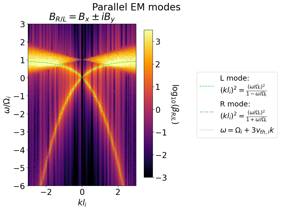
Fig. 9 Calculated Alvén waves spectrum with the theoretical dispersions overlaid.
Perpendicularly propagating modes are also supported, commonly referred to as ion-Bernstein modes.
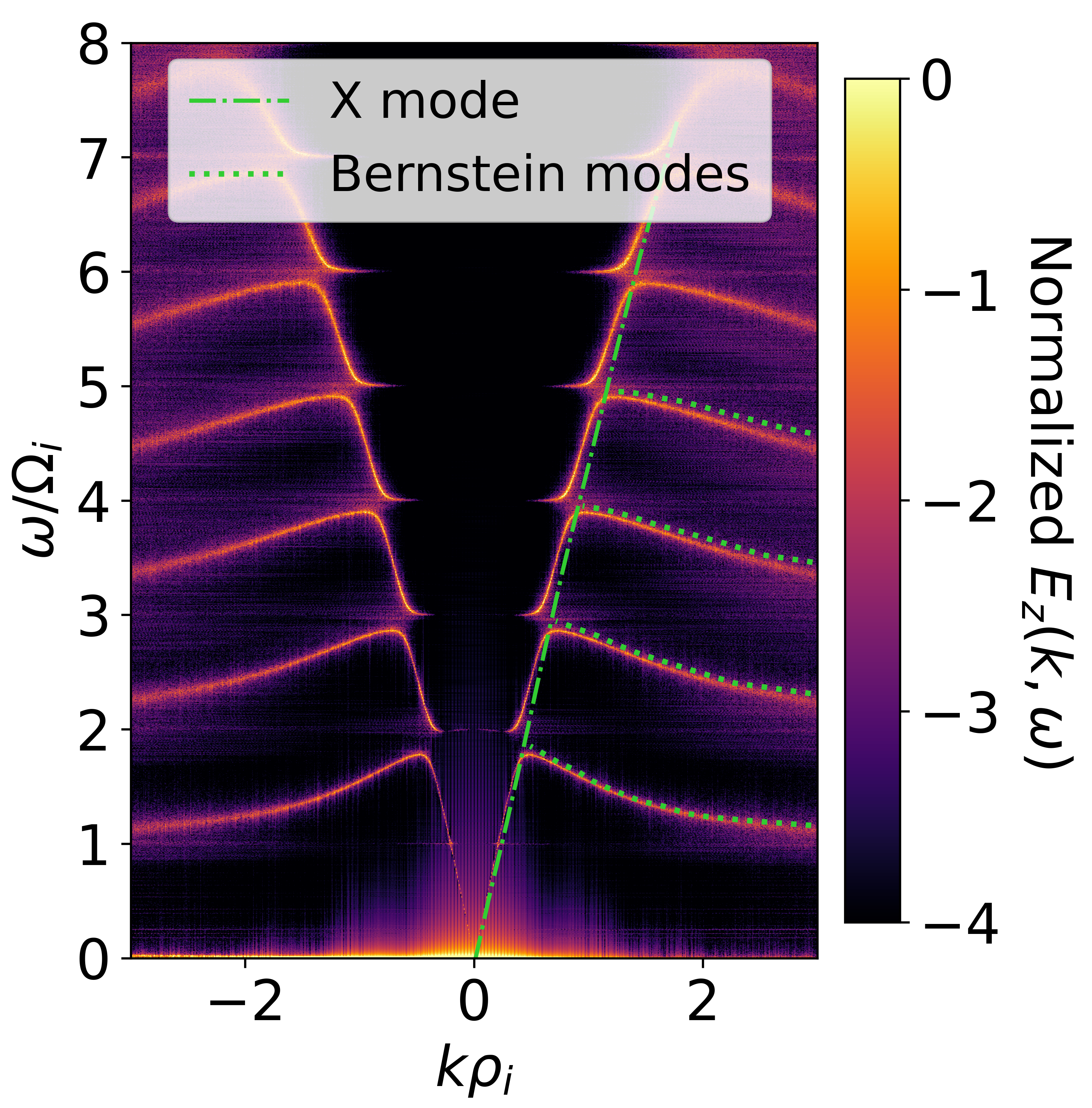
Fig. 10 Calculated ion Bernstein waves spectrum with the theoretical dispersion overlaid.
Ohm solver: Cylindrical normal modes
A RZ-geometry example case for normal modes propagating along an applied magnetic field in a cylinder is also available. The analytical solution for these modes are described in Stix [12] Chapter 6, Sec. 2.
Run
The following script initializes a thermal plasma in a metallic cylinder with periodic boundaries at the cylinder ends.
Script PICMI_inputs_rz.py
#!/usr/bin/env python3
#
# --- Test script for the kinetic-fluid hybrid model in WarpX wherein ions are
# --- treated as kinetic particles and electrons as an isothermal, inertialess
# --- background fluid. The script is set up to produce parallel normal EM modes
# --- in a metallic cylinder and is run in RZ geometry.
# --- As a CI test only a small number of steps are taken.

import argparse
import sys

import dill
import numpy as np
from mpi4py import MPI as mpi
from pywarpx import picmi

constants = picmi.constants

comm = mpi.COMM_WORLD

simulation = picmi.Simulation(verbose=0)


class CylindricalNormalModes(object):
    '''The following runs a simulation of an uniform plasma at a set ion
    temperature (and Te = 0) with an external magnetic field applied in the
    z-direction (parallel to domain).
    The analysis script (in this same directory) analyzes the output field
    data for EM modes.
    '''
    # Applied field parameters
    B0          = 0.5 # Initial magnetic field strength (T)
    beta        = 0.01 # Plasma beta, used to calculate temperature

    # Plasma species parameters
    m_ion       = 400.0 # Ion mass (electron masses)
    vA_over_c   = 5e-3 # ratio of Alfven speed and the speed of light

    # Spatial domain
    Nz          = 512 # number of cells in z direction
    Nr          = 128 # number of cells in r direction

    # Temporal domain (if not run as a CI test)
    LT          = 800.0 # Simulation temporal length (ion cyclotron periods)

    # Numerical parameters
    NPPC        = 8000 # Seed number of particles per cell
    DZ          = 0.4 # Cell size (ion skin depths)
    DR          = 0.4 # Cell size (ion skin depths)
    DT          = 0.02 # Time step (ion cyclotron periods)

    # Plasma resistivity - used to dampen the mode excitation
    eta = 5e-4
    # Number of substeps used to update B
    substeps = 20

    def __init__(self, test, verbose):
        """Get input parameters for the specific case desired."""
        self.test = test
        self.verbose = verbose or self.test

        # calculate various plasma parameters based on the simulation input
        self.get_plasma_quantities()

        if not self.test:
            self.total_steps = int(self.LT / self.DT)
        else:
            # if this is a test case run for only a small number of steps
            self.total_steps = 100
            # and make the grid and particle count smaller
            self.Nz = 128
            self.Nr = 64
            self.NPPC = 200
        # output diagnostics 5 times per cyclotron period
        self.diag_steps = max(10, int(1.0 / 5 / self.DT))

        self.Lz = self.Nz * self.DZ * self.l_i
        self.Lr = self.Nr * self.DR * self.l_i

        self.dt = self.DT * self.t_ci

        # dump all the current attributes to a dill pickle file
        if comm.rank == 0:
            with open(f'sim_parameters.dpkl', 'wb') as f:
                dill.dump(self, f)

        # print out plasma parameters
        if comm.rank == 0:
            print(
                f"Initializing simulation with input parameters:\n"
                f"\tT = {self.T_plasma:.3f} eV\n"
                f"\tn = {self.n_plasma:.1e} m^-3\n"
                f"\tB0 = {self.B0:.2f} T\n"
                f"\tM/m = {self.m_ion:.0f}\n"
            )
            print(
                f"Plasma parameters:\n"
                f"\tl_i = {self.l_i:.1e} m\n"
                f"\tt_ci = {self.t_ci:.1e} s\n"
                f"\tv_ti = {self.v_ti:.1e} m/s\n"
                f"\tvA = {self.vA:.1e} m/s\n"
            )
            print(
                f"Numerical parameters:\n"
                f"\tdt = {self.dt:.1e} s\n"
                f"\tdiag steps = {self.diag_steps:d}\n"
                f"\ttotal steps = {self.total_steps:d}\n",
                flush=True
            )
        self.setup_run()

    def get_plasma_quantities(self):
        """Calculate various plasma parameters based on the simulation input."""
        # Ion mass (kg)
        self.M = self.m_ion * constants.m_e

        # Cyclotron angular frequency (rad/s) and period (s)
        self.w_ci = constants.q_e * abs(self.B0) / self.M
        self.t_ci = 2.0 * np.pi / self.w_ci

        # Alfven speed (m/s): vA = B / sqrt(mu0 * n * (M + m)) = c * omega_ci / w_pi
        self.vA = self.vA_over_c * constants.c
        self.n_plasma = (
            (self.B0 / self.vA)**2 / (constants.mu0 * (self.M + constants.m_e))
        )

        # Ion plasma frequency (Hz)
        self.w_pi = np.sqrt(
            constants.q_e**2 * self.n_plasma / (self.M * constants.ep0)
        )

        # Skin depth (m)
        self.l_i = constants.c / self.w_pi

        # Ion thermal velocity (m/s) from beta = 2 * (v_ti / vA)**2
        self.v_ti = np.sqrt(self.beta / 2.0) * self.vA

        # Temperature (eV) from thermal speed: v_ti = sqrt(kT / M)
        self.T_plasma = self.v_ti**2 * self.M / constants.q_e # eV

        # Larmor radius (m)
        self.rho_i = self.v_ti / self.w_ci

    def setup_run(self):
        """Setup simulation components."""

        #######################################################################
        # Set geometry and boundary conditions                                #
        #######################################################################

        self.grid = picmi.CylindricalGrid(
            number_of_cells=[self.Nr, self.Nz],
            warpx_max_grid_size=self.Nz,
            lower_bound=[0, -self.Lz/2.0],
            upper_bound=[self.Lr, self.Lz/2.0],
            lower_boundary_conditions = ['none', 'periodic'],
            upper_boundary_conditions = ['dirichlet', 'periodic'],
            lower_boundary_conditions_particles = ['absorbing', 'periodic'],
            upper_boundary_conditions_particles = ['reflecting', 'periodic']
        )
        simulation.time_step_size = self.dt
        simulation.max_steps = self.total_steps
        simulation.current_deposition_algo = 'direct'
        simulation.particle_shape = 1
        simulation.verbose = self.verbose

        #######################################################################
        # Field solver and external field                                     #
        #######################################################################

        self.solver = picmi.HybridPICSolver(
            grid=self.grid,
            Te=0.0, n0=self.n_plasma, plasma_resistivity=self.eta,
            substeps=self.substeps,
            n_floor=self.n_plasma*0.05
        )
        simulation.solver = self.solver

        B_ext = picmi.AnalyticInitialField(
            Bz_expression=self.B0
        )
        simulation.add_applied_field(B_ext)

        #######################################################################
        # Particle types setup                                                #
        #######################################################################

        self.ions = picmi.Species(
            name='ions', charge='q_e', mass=self.M,
            initial_distribution=picmi.UniformDistribution(
                density=self.n_plasma,
                rms_velocity=[self.v_ti]*3,
            )
        )
        simulation.add_species(
            self.ions,
            layout=picmi.PseudoRandomLayout(
                grid=self.grid, n_macroparticles_per_cell=self.NPPC
            )
        )

        #######################################################################
        # Add diagnostics                                                     #
        #######################################################################

        field_diag = picmi.FieldDiagnostic(
            name='field_diag',
            grid=self.grid,
            period=self.diag_steps,
            data_list=['B', 'E'],
            write_dir='diags',
            warpx_file_prefix='field_diags',
            warpx_format='openpmd',
            warpx_openpmd_backend='h5',
        )
        simulation.add_diagnostic(field_diag)

        # add particle diagnostic for checksum
        if self.test:
            part_diag = picmi.ParticleDiagnostic(
                name='diag1',
                period=self.total_steps,
                species=[self.ions],
                data_list=['ux', 'uy', 'uz', 'weighting'],
                write_dir='.',
                warpx_file_prefix='Python_ohms_law_solver_EM_modes_rz_plt'
            )
            simulation.add_diagnostic(part_diag)


##########################
# parse input parameters
##########################

parser = argparse.ArgumentParser()
parser.add_argument(
    '-t', '--test', help='toggle whether this script is run as a short CI test',
    action='store_true',
)
parser.add_argument(
    '-v', '--verbose', help='Verbose output', action='store_true',
)
args, left = parser.parse_known_args()
sys.argv = sys.argv[:1]+left

run = CylindricalNormalModes(test=args.test, verbose=args.verbose)
simulation.step()
The example can be executed using:
python3 PICMI_inputs_rz.py
Analyze
After the simulation completes the following script can be used to analyze the field evolution and extract the normal mode dispersion relation. It performs a standard Fourier transform along the cylinder axis and a Hankel transform in the radial direction.
Script analysis_rz.py
#!/usr/bin/env python3
#
# --- Analysis script for the hybrid-PIC example producing EM modes.

import dill
import matplotlib.pyplot as plt
import numpy as np
import scipy.fft as fft
from matplotlib import colors
from openpmd_viewer import OpenPMDTimeSeries
from pywarpx import picmi
from scipy.interpolate import RegularGridInterpolator
from scipy.special import j1, jn, jn_zeros

constants = picmi.constants

# load simulation parameters
with open(f'sim_parameters.dpkl', 'rb') as f:
    sim = dill.load(f)

diag_dir = "diags/field_diags"

ts = OpenPMDTimeSeries(diag_dir, check_all_files=True)

def transform_spatially(data_for_transform):
    # interpolate from regular r-grid to special r-grid
    interp = RegularGridInterpolator(
        (info.z, info.r), data_for_transform,
        method='linear'
    )
    data_interp = interp((zg, rg))

    # Applying manual hankel in r
    # Fmz = np.sum(proj*data_for_transform, axis=(2,3))
    Fmz = np.einsum('ijkl,kl->ij', proj, data_interp)
    # Standard fourier in z
    Fmn = fft.fftshift(fft.fft(Fmz, axis=1), axes=1)
    return Fmn

def process(it):
    print(f"Processing iteration {it}", flush=True)
    field, info = ts.get_field('E', 'y', iteration=it)
    F_k = transform_spatially(field)
    return F_k

# grab the first iteration to get the grids
Bz, info = ts.get_field('B', 'z', iteration=0)

nr = len(info.r)
nz = len(info.z)

nkr = 12 # number of radial modes to solve for

r_max = np.max(info.r)

# create r-grid with points spaced out according to zeros of the Bessel function
r_grid = jn_zeros(1, nr) / jn_zeros(1, nr)[-1] * r_max

zg, rg = np.meshgrid(info.z, r_grid)

# Setup Hankel Transform
j_1M = jn_zeros(1, nr)[-1]
r_modes = np.arange(nkr)

A = (
    4.0 * np.pi * r_max**2 / j_1M**2
    * j1(np.outer(jn_zeros(1, max(r_modes)+1)[r_modes], jn_zeros(1, nr)) / j_1M)
    / jn(2 ,jn_zeros(1, nr))**2
)

# No transformation for z
B = np.identity(nz)

# combine projection arrays
proj = np.einsum('ab,cd->acbd', A, B)

results = np.zeros((len(ts.t), nkr, nz), dtype=complex)
for ii, it in enumerate(ts.iterations):
    results[ii] = process(it)

# now Fourier transform in time
F_kw = fft.fftshift(fft.fft(results, axis=0), axes=0)

dz = info.z[1] - info.z[0]
kz = 2*np.pi*fft.fftshift(fft.fftfreq(F_kw[0].shape[1], dz))
dt = ts.iterations[1] - ts.iterations[0]
omega = 2*np.pi*fft.fftshift(fft.fftfreq(F_kw.shape[0], sim.dt*dt))

# Save data for future plotting purposes
np.savez(
    "diags/spectrograms.npz",
    F_kw=F_kw, dz=dz, kz=kz, dt=dt, omega=omega
)

# plot the resulting dispersions
k = np.linspace(0, 250, 500)
kappa = k * sim.l_i

fig, axes = plt.subplots(2, 2, sharex=True, sharey=True, figsize=(6.75, 5))

vmin = [2e-3, 1.5e-3, 7.5e-4, 5e-4]
vmax = 1.0

# plot m = 1
for ii, m in enumerate([1, 3, 6, 8]):
    ax = axes.flatten()[ii]
    ax.set_title(f"m = {m}", fontsize=11)
    m -= 1
    pm1 = ax.pcolormesh(
        kz*sim.l_i, omega/sim.w_ci,
        abs(F_kw[:, m, :])/np.max(abs(F_kw[:, m, :])),
        norm=colors.LogNorm(vmin=vmin[ii], vmax=vmax),
        cmap='inferno'
    )
    cb = fig.colorbar(pm1, ax=ax)
    cb.set_label(r'Normalized $E_\theta(k_z, m, \omega)$')

    # Get dispersion relation - see for example
    # T. Stix, Waves in Plasmas (American Inst. of Physics, 1992), Chap 6, Sec 2
    nu_m = jn_zeros(1, m+1)[-1] / sim.Lr
    R2 = 0.5 * (nu_m**2 * (1.0 + kappa**2) + k**2 * (kappa**2 + 2.0))
    P4 = k**2 * (nu_m**2 + k**2)
    omega_fast = sim.vA * np.sqrt(R2 + np.sqrt(R2**2 - P4))
    omega_slow = sim.vA * np.sqrt(R2 - np.sqrt(R2**2 - P4))
    # Upper right corner
    ax.plot(k*sim.l_i, omega_fast/sim.w_ci, 'w--', label = f"$\omega_{{fast}}$")
    ax.plot(k*sim.l_i, omega_slow/sim.w_ci, color='white', linestyle='--', label = f"$\omega_{{slow}}$")
    # Thermal resonance
    thermal_res = sim.w_ci + 3*sim.v_ti*k
    ax.plot(k*sim.l_i, thermal_res/sim.w_ci, color='magenta', linestyle='--', label = "$\omega = \Omega_i + 3v_{th,i}k$")
    ax.plot(-k*sim.l_i, thermal_res/sim.w_ci, color='magenta', linestyle='--', label = "")
    thermal_res = sim.w_ci - 3*sim.v_ti*k
    ax.plot(k*sim.l_i, thermal_res/sim.w_ci, color='magenta', linestyle='--', label = "$\omega = \Omega_i + 3v_{th,i}k$")
    ax.plot(-k*sim.l_i, thermal_res/sim.w_ci, color='magenta', linestyle='--', label = "")


for ax in axes.flatten():
    ax.set_xlim(-1.75, 1.75)
    ax.set_ylim(0, 1.6)

axes[0, 0].set_ylabel('$\omega/\Omega_{ci}$')
axes[1, 0].set_ylabel('$\omega/\Omega_{ci}$')
axes[1, 0].set_xlabel('$k_zl_i$')
axes[1, 1].set_xlabel('$k_zl_i$')

plt.savefig('normal_modes_disp.png', dpi=600)
if not sim.test:
    plt.show()
else:
    plt.close()

    # check if power spectrum sampling match earlier results
    amps = np.abs(F_kw[2, 1, len(kz)//2-2:len(kz)//2+2])
    print("Amplitude sample: ", amps)
    assert np.allclose(
        amps, np.array([ 61.02377286,  19.80026021, 100.47687017,  10.83331295])
    )

if sim.test:
    import os
    import sys
    sys.path.insert(1, '../../../../warpx/Regression/Checksum/')
    import checksumAPI

    # this will be the name of the plot file
    fn = sys.argv[1]
    test_name = os.path.split(os.getcwd())[1]
    checksumAPI.evaluate_checksum(test_name, fn, rtol=1e-6)
The following figure was produced with the above analysis script, showing excellent agreement between the calculated and theoretical dispersion relations.
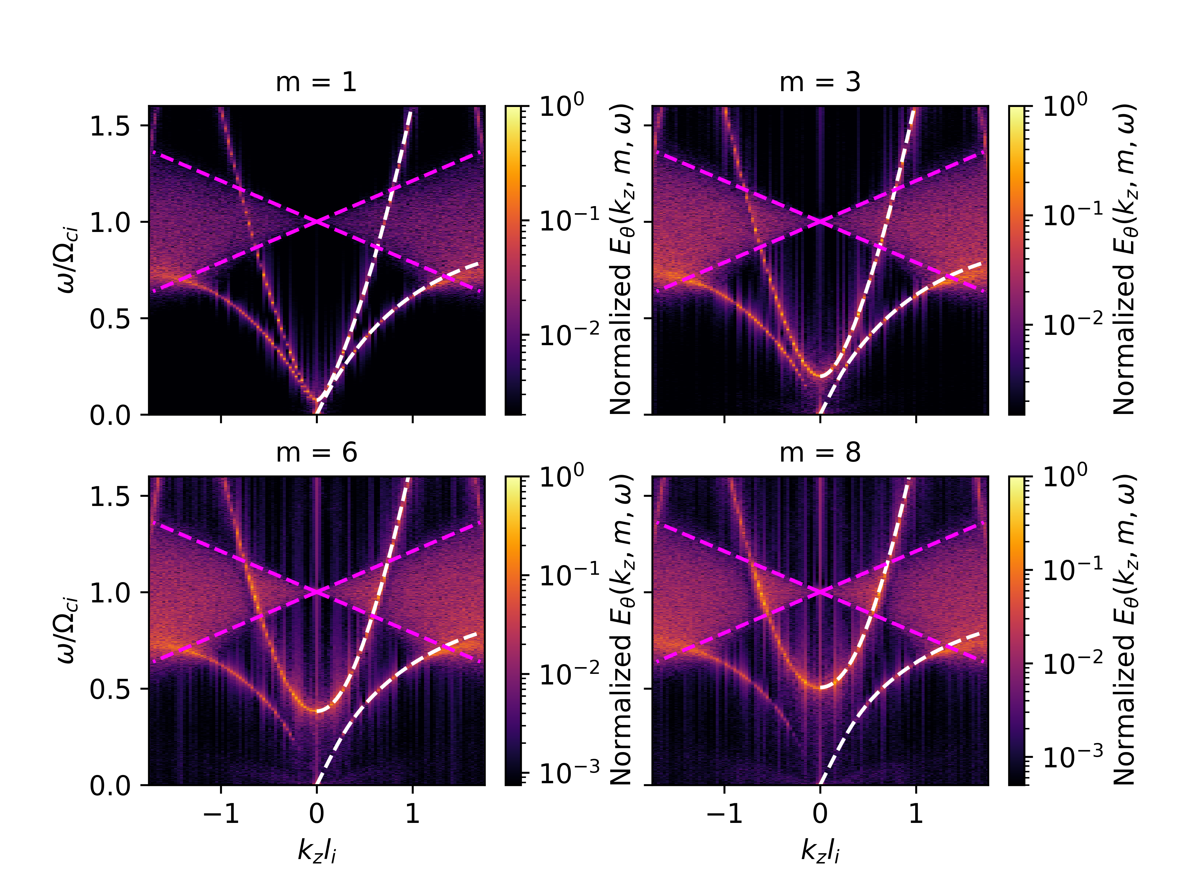
Fig. 11 Cylindrical normal mode dispersion comparing the calculated spectrum with the theoretical one.