Training a Surrogate Model from WarpX Data
Suppose we have a WarpX simulation that we wish to replace with a neural network surrogate model. For example, a simulation determined by the following input script
In this section we walk through a workflow for data processing and model training. This workflow was developed and first presented in Sandberg et al. [1], Sandberg et al. [2].
This assumes you have an up-to-date environment with PyTorch and openPMD.
Data Cleaning
It is important to inspect the data for artifacts to check that input/output data make sense. If we plot the final phase space for beams 1-8, the particle data is distributed in a single blob, as shown by Fig. 15 for beam 1. This is as we expect and what is optimal for training neural networks.
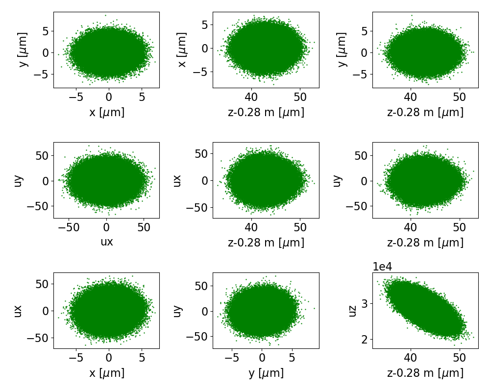
Fig. 15 The final phase space projections for beam 1 of the training data, for a surrogate to stage 1.
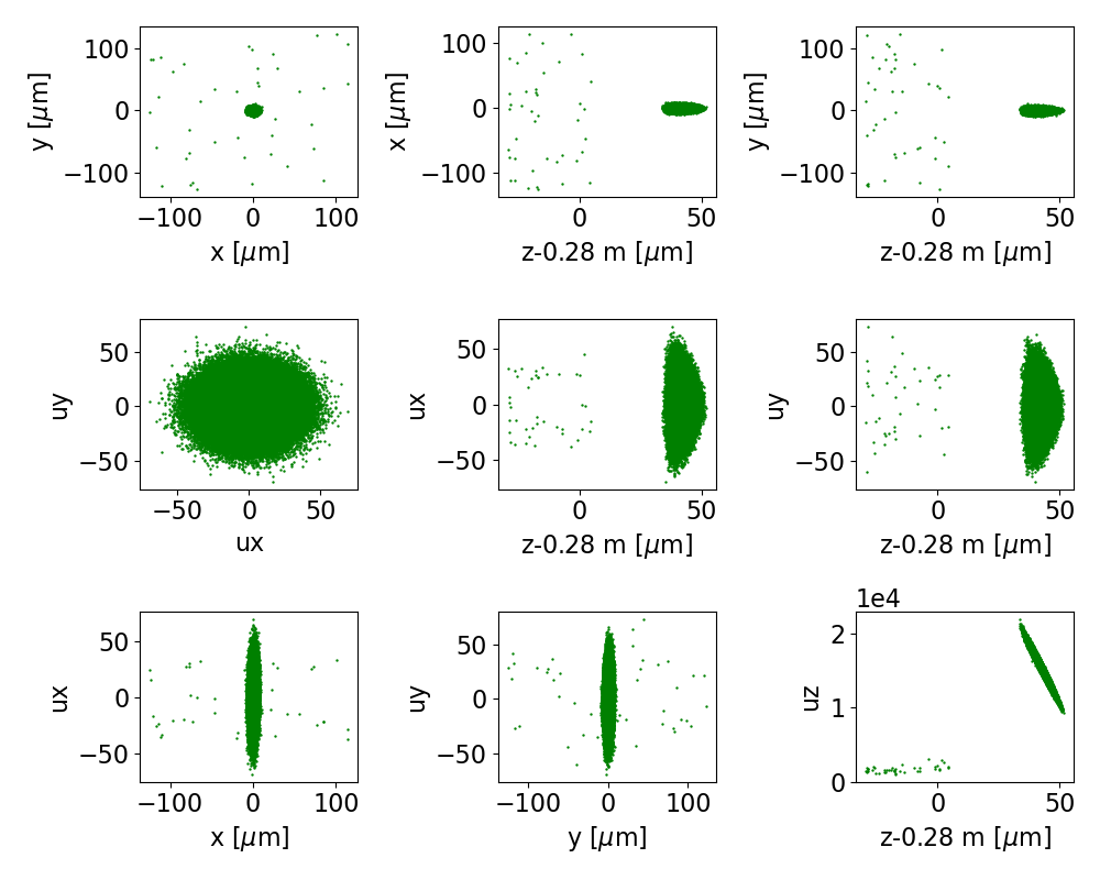
Fig. 16 The final phase space projections for beam 0 of the training data, for a surrogate to stage 0
On the other hand, the final phase space for beam 0, shown in Fig. 15,
has a halo of outlying particles.
Looking closer at the z-pz space, we see that some particles got caught in a decelerating
region of the wake, have slipped back and are much slower than the rest of the beam.
To assist our neural network in learning dynamics of interest, we filter out these particles.
It is sufficient for our purposes to select particles that are not too far back, setting
particle_selection={'z':[0.28002, None]}. Then a particle tracker is set up to make sure
we consistently filter out these particles from both the initial and final data.
iteration = ts.iterations[target_index]
pt = ParticleTracker( ts,
                     species=species,
                     iteration=iteration,
                     select=particle_selection)
Create Normalized Dataset
Having chosen training data we are content with, we now need to format the data, normalize it, and store the normalized data as well as the normalizations. The script below will take the openPMD data we have selected and format, normalize, and store it.
Load openPMD Data
First the openPMD data is loaded, using the particle selector as chosen above. The neural network will make predictions from the initial phase space coordinates, using the final phase space coordinates to measure how well it is making predictions. Hence we load two sets of particle data, the source and target particle arrays.
iteration = ts.iterations[source_index]
source_data = ts.get_particle(species=species,
                              iteration=iteration,
                              var_list=['x','y','z','ux','uy','uz'],
                              select=pt)

iteration = ts.iterations[target_index]
target_data = ts.get_particle(species=species,
                              iteration=iteration,
                              var_list=['x','y','z','ux','uy','uz'],
                              select=pt)
Normalize Data
Neural networks learn better on appropriately normalized data. Here we subtract out the mean in each coordinate direction and divide by the standard deviation in each coordinate direction, for normalized data that is centered on the origin with unit variance.
target_means = np.zeros(6)
target_stds = np.zeros(6)
source_means = np.zeros(6)
source_stds = np.zeros(6)
for jj in range(6):
    source_means[jj] = source_data[jj].mean()
    source_stds[jj] = source_data[jj].std()
    source_data[jj] -= source_means[jj]
    source_data[jj] /= source_stds[jj]

for jj in range(6):
    target_means[jj] = target_data[jj].mean()
    target_stds[jj] = target_data[jj].std()
    target_data[jj] -= target_means[jj]
    target_data[jj] /= target_stds[jj]
openPMD to PyTorch Data
With the data normalized, it must be stored in a form PyTorch recognizes. The openPMD data are 6 lists of arrays, for each of the 6 phase space coordinates \(x, y, z, p_x, p_y,\) and \(p_z\). This data are converted to an \(N\times 6\) numpy array and then to a PyTorch \(N\times 6\) tensor.
source_data = torch.tensor(np.column_stack(source_data))
target_data = torch.tensor(np.column_stack(target_data))
Save Normalizations and Normalized Data
With the data properly normalized, it and the normalizations are saved to file for use in training and inference.
full_dataset = torch.utils.data.TensorDataset(source_data.float(), target_data.float())

n_samples = full_dataset.tensors[0].size(0)
n_train = int(training_frac*n_samples)
n_test = n_samples - n_train

train_data, test_data = torch.utils.data.random_split(full_dataset, [n_train, n_test])

torch.save({'dataset':full_dataset,
            'train_indices':train_data.indices,
            'test_indices':test_data.indices,
            'source_means':source_means,
            'source_stds':source_stds,
            'target_means':target_means,
            'target_stds':target_stds,
            'times':times,
           },
            dataset_fullpath_filename
          )
Neural Network Structure
It was found in Sandberg et al. [2] that reasonable surrogate models are obtained with shallow feedforward neural networks consisting of fewer than 10 hidden layers and just under 1000 nodes per layer. The example shown here uses 3 hidden layers and 20 nodes per layer and is trained for 10 epochs.
Train and Save Neural Network
The script below trains the neural network on the dataset just created. In subsequent sections we discuss the various parts of the training process.
Training Function
In the training function, the model weights are updated.
Iterating through batches, the loss function is evaluated on each batch.
PyTorch provides automatic differentiation, so the direction of steepest descent
is determined when the loss function is evaluated and the loss.backward() function
is invoked.
The optimizer uses this information to update the weights in the optimizer.step() call.
The training loop then resets the optimizer and updates the summed error for the whole dataset
with the error on the batch and continues iterating through batches.
Note that this function returns the sum of all errors across the entire dataset,
which is later divided by the size of the dataset in the training loop.
def train(model, optimizer, train_loader, loss_fun):
    model.train()
    total_loss = 0.
    for batch_idx, (data, target) in enumerate(train_loader):
        #evaluate network with data
        output = model(data)
        #compute loss
         # sum the differences squared, take mean afterward
        loss = loss_fun(output, target,reduction='sum')
        #backpropagation: step optimizer and reset gradients
        loss.backward()
        optimizer.step()
        optimizer.zero_grad()
        total_loss += loss.item()
    return total_loss
Testing Function
The testing function just evaluates the neural network on the testing data that has not been used to update the model parameters. This testing function requires that the testing dataset is small enough to be loaded all at once. The PyTorch dataloader can load data in batches if this size assumption is not satisfied. The error, measured by the loss function, is returned by the testing function to be aggregated and stored. Note that this function returns the sum of all errors across the entire dataset, which is later divided by the size of the dataset in the training loop.
def test_dataset(model, test_source, test_target, loss_fun):
    model.eval()
    with torch.no_grad():
        output = model(test_source)
        return loss_fun(output, test_target, reduction='sum').item()
Train Loop
The full training loop performs n_epochs number of iterations.
At each iteration the training and testing functions are called,
the respective errors are divided by the size of the dataset and recorded,
and a status update is printed to the console.
for epoch in range(n_epochs):
    if do_print:
        t1 = time.time()
    ave_train_loss = train(model, optimizer, train_loader_device, loss_fun) / data_dim / training_set_size
    ave_test_loss = test_dataset(model, test_source_device, test_target_device, loss_fun)  / data_dim / training_set_size
    train_loss_list.append(ave_train_loss)
    test_loss_list.append(ave_test_loss)

    if do_print:
        t2 = time.time()
        print('Train Epoch: {:04d} \tTrain Loss: {:.6f} \tTest Loss: {:.6f}, this epoch: {:.3f} s'.format(
                epoch + 1, ave_train_loss, ave_test_loss, t2-t1))
Save Neural Network Parameters
The model weights are saved after training to record the updates to the model parameters. Additionally, we save some model metainformation with the model for convenience, including the model hyperparameters, the training and testing losses, and how long the training took.
model.to(device='cpu')
torch.save({
    'n_hidden_layers':n_hidden_layers,
    'n_hidden_nodes':n_hidden_nodes,
    'activation':activation_type,
    'model_state_dict': model.state_dict(),
    'optimizer_state_dict': optimizer.state_dict(),
    'train_loss_list': train_loss_list,
    'test_loss_list': test_loss_list,
    'training_time': training_time,
    }, f'models/{species}_model.pt')
Evaluate
In this section we show two ways to diagnose how well the neural network is learning the data. First we consider the train-test loss curves, shown in Fig. 17. This figure shows the model error on the training data (in blue) and testing data (in green) as a function of the number of epochs seen. The training data is used to update the model parameters, so training error should be lower than testing error. A key feature to look for in the train-test loss curve is the inflection point in the test loss trend. The testing data is set aside as a sample of data the neural network hasn’t seen before. The testing error serves as a metric of model generalizability, indicating how well the model performs on data it hasn’t seen yet. When the test-loss starts to trend flat or even upward, the neural network is no longer improving its ability to generalize to new data.
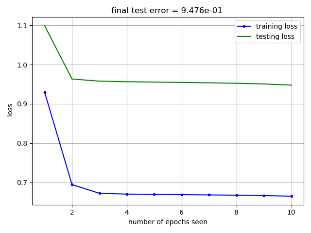
Fig. 17 Training (in blue) and testing (in green) loss curves versus number of training epochs.
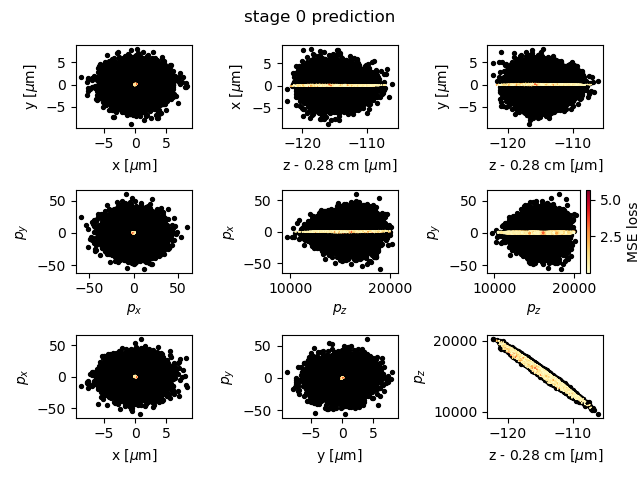
Fig. 18 A comparison of model prediction (yellow-red dots, colored by mean-squared error) with simulation output (black dots).
A visual inspection of the model prediction can be seen in Fig. 18. This plot compares the model prediction, with dots colored by mean-square error, on the testing data with the actual simulation output in black. The model obtained with the hyperparameters chosen here trains quickly but is not very accurate. A more accurate model is obtained with 5 hidden layers and 800 nodes per layer, as discussed in Sandberg et al. [2].
These figures can be generated with the following Python script.
Surrogate Usage in Accelerator Physics
A neural network such as the one we trained here can be incorporated in other BLAST codes. Consider the example using neural networks in ImpactX.
R. Sandberg, R. Lehe, C. E. Mitchell, M. Garten, J. Qiang, J.-L. Vay, and A. Huebl. Hybrid beamline element ML-training for surrogates in the ImpactX beam-dynamics code. In Proc. 14th International Particle Accelerator Conference, number 14 in IPAC'23 - 14th International Particle Accelerator Conference, 2885–2888. Venice, Italy, May 2023. JACoW Publishing, Geneva, Switzerland. URL: https://indico.jacow.org/event/41/contributions/2276, doi:10.18429/JACoW-IPAC2023-WEPA101.